Marginalized Forex Daytrading Strategy: An Application of the Gaussian Mixture Model, Hidden Markov Model, and Johnson's Su Model to Marginalized Currency Pairs

Forex Daytrading Strategy : An Application of the Gaussian Mixture Model to Marginalized Currency pairs in Africa

Stratégie en Daytrading sur le Forex: Une Application du Modèle de Mélange Gaussien aux Paires de Devises Marginalisées en Afrique

Yvan Jorel Ngaleu Ngoyi, PhD in Scientific Algorithmic Trading, E-mail: official@refonteinfini.com 

ElieNNgongang, Professor of Economics and Quantitative Techniques, Email: ngongother@yahoo.fr                                                                                                                                                                                                                                   

Abstract: In this article, we build a Daytrading strategy by applying a Gaussian Mixture Model (GMM) to so-called “marginalized” African currency pairs. With a sample of data covering the period of 01/01/2010 to 05/15/2021 and downloaded in real time from the US Federal Reserve (FRED) website and the Yahoo Finance platform, we found that by including four explanatory variables in the Gaussian mixture model, the GMM independently estimates the returns of the following six African currency pairs with an average accuracy of approximately 56.379%: USDZAR, USDNGN, USDEGP, USDMAD, USDMUR and USDKES. The accuracy of the estimations obtained with the GMM on the returns of the USDZAR currency pair is the highest (73.887%) among the six currency pairs studied in this work. Based on the above results, we have built a trading robot (based on the GMM) that runs in real time and which we have deployed in production in the exchange rate market. In general, by adjusting several parameters of the GMM, our trading robot achieves overall positive daily gains.

Résumé : Dans cet article, nous construisons une stratégie en Daytrading en appliquant un modèle de mélange gaussien (GMM) aux paires de devises africaines dites « marginalisées ». Avec un échantillon de données s’étalant sur la période 01/01/2010 à 15/05/2021 et téléchargé en temps réel sur le site de la Reserve Fédérale Américaine (FRED) et la plateforme Yahoo Finance, nous avons constaté qu’en incluant quatre variables explicatives dans le modèle de mélange gaussien, le GMM estime indépendamment les rendements des six paires de devises africaines suivantes avec une précision moyenne d’environ 56,379% : USDZAR, USDNGN, USDEGP, USDMAD, USDMUR et USDKES. La précision des estimations obtenues avec le GMM sur les rendements de la paire de devise USDZAR est la plus élevée (73,887%) parmi les six paires de devises étudiées dans ce travail. Fort des résultats ci-dessus, nous avons construit un robot de trading (à partir du GMM) qui tourne en temps réel et que nous avons déployé en production sur le marché des taux de changes. De manière générale, en ajustant plusieurs paramètres du GMM, notre robot de trading obtient des gains journaliers globalement positifs.

Keywords: Strategy, Daytrading, GMM, so-called “marginalized” currency pairs, trading robot.

Mots clés : Stratégie, Daytrading, GMM, paires de devises dites « marginalisées », robot de trading.

Introduction

New financial assets have appeared in the last ten years on the currency market (Forex). These new assets generally concern the parity between major currencies^[1] and popular cryptocurrencies.^[2] Cryptocurrencies today have an insignificant influence on the currency market.  Indeed, the volume of transactions on cryptocurrencies is much lower than that on Forex (reminder: the daily trading volume on Forex is about 6600 billion US dollars) . It is very important to study the new joint ecosystem in which exchange rates and cryptocurrencies are bathed. A good anticipation of the future of exchange rates and digital currencies can lead to investment opportunities and may also prevent drifts (crises, bubbles) that may arise from these new currencies.

The objective of this article is to construct a daily strategy, based on the Gaussian Mixture Model (GMM), serving as an algorithmic trading tool for participants in the currency market. In other words, our objective in this article is to build a trading robot that runs in real time around the clock from the GMM and anticipates the evolution of returns on African currency pairs. Several financial firms are interested in trading robots and/or the empirical validation of models that they can use as a basis to develop a trading algorithm that they will then connect to the market to increase their returns. We can cite, for example, the companies Quantiacs and QuantConnect, which receive the models developed and programmed by any researcher, connect them to the market, and share the profits with the researcher if the model is profitable.

The stationarity hypothesis is regularly violated when applied to financial product data. The violation of this assumption in financial markets renders almost all autoregressive models (including ARCH and GARCH family models) ineffective in anticipating and/or predicting stock price movements (Wang et al, 2019).

Long forgotten by scientists, parametric models have flourished over the last twenty years thanks to the exponential growth in the computing power of machine processors, the increase in the size of machine memory, the increase in machine disk space and the democratization (lower prices) of machines (servers, laptops,  mobile phones, ...). This phenomenon is empirically observable by Gordon Moore's first and second laws (1965). This observation also shows us that most parametric models that have many parameters and require good computing power (unless we want to run a simulation/calculation and wait a few days to get the outputs) can now be computer by everyone from the moment we have a laptop or a mobile phone. Thus, in this article, we propose to use the Gaussian Mixture Model  (GMM (1894)) and the  Hidden Markov Model (HMM), both accompanied by the Johnson Su model (1949), to build a Forex trading robot capable of opening one or more positions in a day,  take profits, and close those positions on the same day. In other words, it is about building a Daytrading strategy on Forex by applying the Gaussian mix model to African currency pairs. s

The contribution of this article is a first: unless we are mistaken, and after having gone through the financial literature, we think that it is a first time in the financial literature that a robot built from the GMM-HMM^[3] and trade on African currency pairs (and running in real time 24 hours a day on the Forex market) has been developed, coded, and published by researchers. The estimates of the parameters of the robot using the GMM-HMM were made from a sample of data extending over the period 01/01/2010 to 15/05/2021 and downloaded in real time from the website of the US Federal Reserve (FRED) and the Yahoo Finance platform.  The remainder of the article is organized as follows: section (1) presents the literature review; section (2) discusses research questions and hypotheses; section (3) describes the methodological approach; section (4) presents and discusses the results.

1. Financial Markets Literature Review

Financial markets are the markets in which short-, medium- and long-term demand and supply of capital meet. They are also markets in which individuals, private companies and public institutions intervene to trade, buy and/or sell financial securities.

In this section 1, we present on the one hand the context and the review of the literature, i.e. the microstructure of the foreign exchange market, the different participants in the Forex market and the different types of algorithmic trading; On the other hand,  we present a review of the literature on models commonly used in financial markets, i.e.  we review the scientific literature on linear models and nonlinear or probabilistic models generally used in finance.

1.1 Background and literature review

Financial markets are markets in which individuals,  private companies and public institutions can trade securities, commodities and other assets at prices that reflect supply and demand^[4].

The foreign exchange market is the market in which all participants who want to sell or buy one currency in exchange for another currency meet. Transactions on the foreign exchange market have increased by more than a third over the last three years, reaching 6.6trillion dollars (more than 5,400 billion euros) per day, or about 90% of Japan's annual GDP (Bank of International Settlement, 2004 and 2019).

The presence of trends and volatility in the foreign exchange markets between 2001 and 2004 led to an increase in commercial dynamism, where investors took large positions in foreign currency. This then led to an appreciation of trends and short positions by decreasing currencies.  This decline in currencies has squeezed economic activity. To this end, most central banks have responded by increasing liquidity in the economy. These trends have also led to an increase in hedging activities against exchange rate fluctuations (Idvall et al, 2008).

On the Forex, there are six main players to varying degrees: commercial banks, institutional investors, multinational enterprises, central banks, brokers and individuals (Idvall 2008 , Guerreiro 2016).

The Forex market can be organized into two main compartments: the interbank market and the foreign exchange market open to the rest of the world. Interbank market transactions take place between central banks and commercial banks (Guerreiro, 2016).

Foreign exchange markets are often called "commercial" or "dematerialized" because of their electronic nature: they take the form of computer networks between financial institutions.  The Nasdaq was one of the first over-the-counter markets where technology replaced the physical interaction of humans (Hendershott, 2003).

With the boom in technological advancements in the finance industry, algorithmic trading (TA) and high frequency trading (HFT) are welcome and accepted for trading anywhere in the world. Within a decade, TA and HFT will be the most common means of trading in developed markets and will spread rapidly in developing economies.

In discretionary trading, the maximum risk comes from decisions made under the influence of the trader’s uncontrolled emotions. In most cases, these emotions can lead to decisions that cannot be logically justified. Therefore, in order to make a profit, it becomes extremely important to not only have a profitable strategy, but also to have control over one's emotions (Kabbaj, 2011).

(Eriksson 2007; Moore 2017) Algorithmic trading means turning a trading idea into a trading strategy via an algorithm. The trading strategy thus created can be "backtested"^[5]  with historical data to check if it will give good returns on real markets. The algorithmic trading strategy can be executed manually or automatically.  Thus, algo traders use algorithms to make buy/sell decisions or to optimize their luck in order to make a profit on the investments they make. The algorithms are modified according to market conditions, type of financial instruments, etc.

Quantitative trading involves using mathematical models   and advanced statistics for the creation and execution of trading strategies. The mission of "quants" is the mathematical modeling of trading strategies.

Automatic trading means that order generation, submission and order execution process are completely automatic.

Trading strategies can be categorized into low frequency, medium frequency, and high frequency strategies depending on how long orders are held. High frequency strategies are algorithmic strategies that are executed in an automated manner in the blink of an eye, usually on a timescale of seconds. These strategies hold their positions for a very short time and try to take advantage of very small profit spreads per trade. These strategies also involve executing millions of trades every day. In other words, the THF is the TA where orders are made at the speed of light (about 1 nanosecond), for purely speculative purposes and positions are closed before the stock market closes. THF and TA can be considered daytrading strategies. As we will see below, daytrading consists of taking positions on average time units and closing your position at the end of the day (i.e. before 24 hours).

Machine Learning and Deep Learning Trading (Moore, 2017): There is sometimes confusion between Artificial Intelligence (AI), Machine Learning (ML) and deep learning or Deep Learning (DL). AI is a much larger space that spans ML and DL. While ML is a part of AI, DL is a subset of ML.

All of these applications are based on the concept of learning from past data and predicting the outcome of a new and unseen situation whose true value will be incorporated into the database and so on; This is done the same way humans learn.

Behind all these trading strategies, there are statistical and econometric models such as linear regression models, multidimensional statistical models (principal component analysis, factorial analysis of correspondences, etc.), autoregressive models (ARMA, ARCH, GARCH) , mixture models (Gaussian mixture models, binomial mixture model, …), Markov models. The Gaussian mixture model is a particular model because it can model any data set but with a random margin of error (Attar, 2012). It is a model that is both additive and multiplicative in the sense that it is a sum of Gaussian models each modeling a cluster, each being assigned a weight (probability) which determines the individual importance of each cluster in the set of data. This robustness of the Gaussian Mixture Model (GMM) is one of the reasons that motivated us to apply the GMM to Forex data.

Depending on the time units on which the Forex players trade, we can group the strategies of these investors into three categories: "scalping" consists of taking positions on very short time frame units (less than 5 minutes ) and stay there for a few minutes; “daytrading” consists of taking positions on average time units and closing your position at the end of the day (i.e. before 24 hours) (Thukral et al, 2013); “swing trading” consists of taking positions on long time frames (between 4 hours and 1 day) and staying there for a few days (Thukral et al, 2013).

The microstructure of financial markets is one of the branches of microeconomics that studies the mechanisms by which prices are formed and influence the market. This discipline is based on the development of mathematical models to determine prices. German (1976) is one of the first authors to work on the microstructure of financial markets. He considers market activity to be a stochastic process that follows a Poisson law. Its objective is to describe the microstructure of financial markets over time. The author then develops two models which are still used today to determine the implications of prices on the markets: one of the models considers that the market is purely price-driven (absence of market-makers or market-makers) and the other considers a market in which prices are centralized at the level of market makers. Demsetz (1968) was the first to research the determinants of transaction costs in financial markets. His study applies data from the New York Stock Exchange (NYSE) because he considers that the NYSE is the largest stock exchange in the world. The objective of his article is to determine the explanatory variables that influence the spread (bid/ask) and to measure the influence that brokerage intermediaries could have on the distribution of transactions and prices. From the time series of the share prices of each company listed on the NYSE, Demetz (1968) constructs a multivariate econometric process. He finds a negative and significant relationship between the distribution of transactions and the size of the market maker; The size of the market maker being measured according to its own funds. It also identifies three sources of costs: order processing costs, inventory holding costs and information asymmetry costs.

The variation of the Spread often leads to costs called "Slippage" which is the difference in cost between the one at which the order would like to be executed and the one where it was actually executed. This can be a problem when you want to get out quickly or if you have small goals (stop loss^[6] and take profit^[7]).  Stop loss and take profit have their origins and justifications in the theories of behavioral finance, led by Daniel Kahneman (1981).  From laboratory experiments, Daniel Kahneman  and Amos Tversky show in 1979 how individuals asymmetrically evaluate their expectations of loss and gain.  To give a very simplified example, the pain of losing  an amount X (e.g. 1000 euros) could only be offset by the pleasure of winning kX (e.g. 2000, or even 3000 euros).^[8] This implies that when a trader is in a loss situation, he tends to lose more and more because he hopes that the  situation will turn around and that when he wins, he tends to take his gains quickly because he does not bear the loss. Two minimal solutions to these psychological biases are on the one hand stop loss and take profit and on the other hand TA and HFT. These psychological biases amplify volatility and clustering in markets (Kabbaj, 2011).

Information (that which has a direct impact on the value of an asset such as economic information) also plays an important role in the behavior of market participants. John Muth (1961) was the first author who introduced the theory of rational expectations to take into account the influence of information in negotiations between economic agents, especially when studying how a large number of individuals, d companies and organizations make choices under uncertainty. But it was Robert Lucas who would make this theory popular in the 1970s when he used it to critique monetarist and Keynesian theories of business cycles; This critique is generally known as the "Lucas Critique". Lucas' idea is that economic agents can very well exploit past and present information to make rational anticipations and make good decisions, so that on average, they are not wrong. In other words, agents can well anticipate the evolution of economic quantities according to their conditional expectations and known information. This does not mean that individuals are perfect preachers or that they are omniscient but that they have the same information. But, still during the 1970s, Akerlof (1970) shows on a second-hand car market that information is not perfect on the markets because there are insider trading, anti- selection and moral hazard. This presence of information asymmetry in the markets has also been studied by Joseph Stiglitz^[9] in the context of market imperfections in economics. This means that information is imperfect in the markets because there are also costs associated with obtaining information. A well-informed investor has an advantage over an uninformed investor because the well-informed investor can better anticipate and, thus, he can minimize his risks and increase his return. Investors looking for the right information on the markets will create a mimicry effect which consists, for an operator, in the imitation of his environment. This effect generates a kind of crowd psychology in the market that follows the law of large numbers because if the vast majority of investors believe that the price of an asset will increase, then this price will increase.

Another Nobel laureate who also worked on information is Eugène Fama (1970). His work on the determination of asset prices earned him the Nobel Prize in 2013. He developed the concept of "efficiency of financial markets" which dates back to the theory of efficient markets of Louis Bachelier (1900). According to Fama, a market is said to be efficient if the prices fully reflect the information available on the market at all times.

According to Brealey et al (2006), the hypothesis of market efficiency implies: we must always take into account the intrinsic variable (or economic variable) that affects the price of a share, and we must not be satisfied only with asset prices and price memory. The first implication is very interesting because it will allow us to take economic variables into account in our model. We then construct a Gaussian mixture model (GMM) in which we introduce both the returns (time series of returns) of the exchange rates and the fundamental macroeconomic variables that have significant effects on the rates (we rely on the literature theoretical and empirical to choose these fundamental variables).

1.2 Literature review of models generally used in financial markets

This article is part of a capitalist and purely selfish economic current to the Adam Smith (Adam Smith: Theory of Moral Sentiments, 1759). "As selfish as man may be supposed, there are evidently certain principles in his nature which lead him to interest himself in the fortunes of others, and which make their happiness necessary to him, although he derives nothing from them. other than the pleasure of seeing them happy" (Adam Smith: Theory of Moral Sentiments, 1759; translate in French by Biziou, Gautier, Pradeau, PUF, Quadrige, 1999, p. 23). It is not because this article is capitalistic that it does not contribute to the very good development of society. The individual (or the company or the bank or the institution or the state) who will apply the GMM model developed in this article (to his currency portfolio on the Forex market) will generate profits which he can then spend or invest in his country; this expenditure will have a more or less negligible positive impact on the overall consumption of the country, which in turn has a positive impact on growth and therefore on the development of the country.

The formal and serious analysis of the risk/return couple was first proposed in 1952 by Markowitz. Following the work of Markowitz, Sharpe proposed in 1964 a complementary model to Markowitz's analysis. The model proposed by Sharpe is known as the “Capital Asset Pricing Model or CAPM” or, in French, “Modèle d’Equilibre des Actifs Financiers ou MEDAF”. This model determines the relationship between the expected return of an investment and the return of the market portfolio or systematic risk or risk that cannot be diversified. In 1976, Ross proposed a multifactorial CAPM approach. This approach of Ross assumes that the return of an asset is explained by several factors and not just a single factor (the profitability of the market portfolio) as thought by Sharpe (1964). This also means that the risk associated with an investment comes from several sources and therefore the CAPM contains several sources of systematic risk. Ross's (1976) model is known as Arbitrage Pricing Theory or "APT".

The Markowitz model (1952) measures the expected return of an asset and the associated risk. The CAPM or in French “MEDAF” is in a way a linear regression of the return on the asset on a single explanatory variable (the return on the market portfolio). The Arbitrage Pricing Theory (APT) is a generalization of the CAPM because in the APT, several factors explain the profitability of the assets and each of them constitutes a source of systematic risk. These models are unrealistic because they are based on several assumptions. For example, the assumption on the independence of residuals is not entirely realistic because in a market there are often correlations between prices.

Despite these limits, the CAPM and the APT remain important for modeling the profitability of financial assets because they can be associated, for example, with autoregressive models (to build, for example, ARMAX) and probabilistic models (to, for example, build latent models of probit, logit, Markov models).

Two papers published in 1927 paved the way for autoregressive processes and moving averages: the paper by Yule (1927) ('On the method of investigating periodicities in disturbed series with sepcial reference to Wolfer's sunspot numbers') and that by Slutzy ( 1927) ('the summation of random causes as the source of cyclical processes'). The prices of the different stock prices are supposed to reflect all the market information and we can therefore treat the time series of the prices of the different stock prices as autoregressive processes. The fact that prices always reflect the information available in a market was first called “financial market efficiency” by Eugène Fama (1970). Fama traces what he calls the "theory", or the "hypothesis", of "efficient financial markets" to Louis Bachelier (1900). The vague formulation he gives to this "theory" ("a market in which prices 'fully reflect' and always the available information is called efficient") had the consequence that it gave rise to (at least) two very different interpretations. On the one hand, a market would be "efficient" if the price of securities follows a random walk, making its evolution unpredictable (this also means that we cannot beat the financial markets); on the other hand, a market would be "efficient" if the price of securities corresponds to their "fundamental" or "intrinsic" value, thus allowing an optimal allocation of resources.                        

In the case where an autoregressive process  is not stationary, it can be stationarized using the primary difference filters (Monbet, 2011).

Sometimes there are seasonal effects in a series; These effects can then be taken into account in the AR model using several methods (Charpentier 2011; Monbet 2011).

Let us consider again our time series;  An MA model is any model written in the form  where  ; ; is white noise.

ARMA (Autoregressive Moving Average) models were first proposed by Box and Jenkins. This is why ARMA models are also called Box-Jenkins models. The autoregressive and moving average models are a combination of the AR models and the MA models.

The AR, MA, ARMA, ARIMA, SARIMA, ARMAX models are based on the assumption of stationarity. But in reality, in financial markets (including currency markets), we notice that the series of stock price returns is not always stationary (Broze, 2016).

One way to challenge this hypothesis is to say that financial returns are not stationary and therefore the residues do not follow the movement of white noise.

Another way to look at it is to say: Even if we force the mean of the residuals to be constant, autocovariances (and autocorrelations) are non-zero. The individual test of nullity of autocorrelations and the global test of nullity of autocorrelations (Statistics of Box-Pierce (1970) and Ljung-Box (1978)) of residues show that these are autocorrelated; This means that  : heteroscedasticity is also said to exist between the residues. So there would be a functional link between the residues: this is probably one of the reasons that motivated Robet Engel in 1982 to imagine the ARCH model (AutoRegressive Conditional Heteroskedasticity). This model takes into account the heteroscedasticity caused by volatility packages in financial markets.  The Generalized ARCH (GARCH) model is a generalized model of the ARCH model. We also speak of Integrated GARCH  (or IGARCH) when the sum of the coefficients of the GARCH model  is equal to 1.

Among the drawbacks of the models of the GARCH family, we can note on the one hand that the response of the conditional variance to innovations is linear (but in reality, innovations do not always follow a linear process) and on the other hand that the distribution tails produced by the GARCH model are too thick compared to the reality observed on the markets (Fauth, 2012).

One of the solutions consists in turning to other probabilistic models such as the regime-switching Markov models introduced by Hamilton (1989).

In these models, it is often assumed that there are dynamic mechanisms in the series of returns that cause the series to "jump" from one regime to another as it moves. This means that, on the series of yields, there are places where the series is stationary and suddenly, a mechanism appears which causes the movement to deviate from the general shape of its trajectory. This kind of abrupt change of regime appears several times on the trajectory of the yield. The origin of these sudden changes may be due to variables exogenous to the model which have effects on the series of returns or to stochastic mechanisms which are themselves in the series of returns Cai (1994).

The Markov model assumes that the variable at t depends only on the variable at t-1; This means that the Markov model assumes that there are only first-order autocorrelations; However, in the financial markets, we sometimes observe autocorrelations of order greater than one. The hidden Markov model assumes that the hidden variables are not observable, but in the economy and on the markets, we can observe and measure the hidden or fundamental variables (Gross Domestic Product, inflation, etc.). Gaussian, probit and/or logit models are often used to calculate the probability that a stock price will be bullish or bearish.

The normal distribution is characterized by: a statistically zero mean, a median equal to the mean, a zero asymmetry coefficient (or in English skewness) and a coefficient of flattening (or in English kurtosis) measuring the thickness of the tails of distribution is equal to 3 (and consequently the excess of kurtosis of a Gaussian distribution is equal to 0). However, on the financial markets, we notice that the series of stock prices violates these four properties of a Gaussian distribution. This means that the average of stock returns is not zero and that it is also different from the median. Similarly, the stock price skewness is different from zero and the excess kurtosis is well above zero.

Despite all these limitations, the Gaussian distribution can be useful if we consider that the series of returns is made up of several clusters and that the returns of each cluster follow a normal distribution: this approach gives rise to the Gaussian mixture model (GMM) . The Gaussian mixture model is for this purpose a weighted sum of several Gaussians, each weighted Gaussian representing the distribution of the returns of each cluster. The weights or weights of the clusters represent the importance of each cluster in the overall series of returns. The GMM and the Hidden Markov Model (HMM) are often used together in a trading strategy to account for predictions of future patterns of returns and regime shifts in the series of those returns, respectively. This association gives rise to the GMM-HMM model that we use in this article.

When no model is adequate for the dataset, a mixture model can be used; Particularly the Gaussian mixture model as it can model any dataset with uncertain accuracy (Vanderplas 2016; Thukral et al 2013).

Mixture models have several applications such as forecasting stock price returns and exchange rates.

2.  Research Issues and Hypotheses

Forecasting the return on an asset is not easy. Traditional time series techniques don't always work well for predicting the performance of an asset. One important reason is that older time series analysis models require the data to be stationary. If it is not stationary, we must transform the data until it becomes stationary: this poses a problem. In practice, several phenomena are observed that violate stationarity rules, including nonlinear processes, seasonality, autocorrelation, and volatility clustering. This renders most traditional models ineffective for our purposes.

2.1 Issues

Hansen (1982) already showed that the estimators of the generalized model of moments were strongly convergent and asymptotic, under the assumption that the observable variables are stationary and ergodic. The GMM being a model of the family of generalized moments, we use it in this study to predict the evolution of African currency pairs. In other words, our objective in this article is to build a trading robot that runs in real time around the clock from the GMM and anticipates the evolution of returns on African currency pairs. We also integrate the HMM model in our robot to take into account changes in Forex regimes. The variables taken into account in our robot are on the one hand the past returns of the African currency pairs and on the other hand, the macroeconomic variables. The signal to buy or sell one currency pair against another is triggered by the so-called “mean reversion” strategy. Many financial firms are interested in trading robots and/or empirically validating models that they can use as a basis for developing a trading algorithm.

With the strong growth of TA and THF on the financial markets, it is increasingly difficult for the old models developed in the literature to anticipate trend reversals on the markets. With algorithms moving at the speed of light in the financial markets, this way of combining the ARMA and ARCH-family models is no longer efficient enough. Since it is a question of our days of light, some authors then thought of models that predict the movement of elementary particles (photons) of it (Zhang et al, 2001). The best known of these models are the hidden Markov models (MMC) or hidden Markov model (HMM) which are massively used in particular in pattern recognition (imaging), in artificial intelligence or in automatic processing of natural language (acoustics).

2.2 GMM and return assumptions

GMM Assumptions: We assume that the GMM is flexible enough to: (1) accommodate non-stationary processes and (2) provide a reasonable approximation of the non-linear process generated by Forex data. We also assume in this article that:

• The best known mixture model is the Gaussian mixture model (GMM). It will then be used for our study as indicated by the theme of our study;
• The GMM assumes that each regime (component, class, state) is generated by a Gaussian process with parameters to be determined;
• The GMM uses the E-M algorithm which alternates between estimating the parameters of the regimes (mean, variance) and the likelihood that these parameters could reconstruct the initial data, until there is convergence or another stopping criterion is met;
• We will initialize the GMM with three components;
• The trading strategy will use a total of 4 factors (or intrinsic macroeconomic variables) to estimate the sequence of each regime and their parameters.

Mixture models in general and GMM in particular have potential. First, they are based on several well-established concepts. An easy way to apply mixture models to properly anticipate asset returns is to view asset returns as a sequence of states or regimes. Each regime is characterized by its own descriptive statistics including average and volatility. Said regimes must for example include low volatility and high volatility. The assumption of the underlying model is that each regime is generated by a Gaussian process with parameters, which we can estimate. The GMM uses an expectation-maximization algorithm to estimate the regime parameters and the highest probability of the sequence of regimes.

Return Assumptions: Given the volatility of the return series in FX markets, we need a model that does not assume that the data is stationary. Our model must also estimate non-linear data. Gaussian mixture models seem to be quite soft and flexible in modeling the movement of exchange rate returns because the GMM can model any given game with uncertain accuracy (ZeljkoIvezic 2014, Attar 2012).

In this article, we assume that:

• Future exchange rates of one currency against another depend on past exchange rates and Forex returns follow a non-stationary process.
• There is a relationship between African currencies and US interest rates, treasury bonds, US inflation.
• Currency pairs in Forex do not follow a random walk. Tests for the absence of a random walk on stock prices are generally made by Markov chains and the Wald-Wolfowitz test (1940). This hypothesis allows us to reassure ourselves of the inefficiency of the financial markets, in particular the Forex market. This inefficiency of the currency market reassures us that the African currency pairs on which we trade are anticipable, predictable and capable of generating us good profits if we correctly predict their future evolutions.
• We also make the assumption that the Forex currency pair datasets follow a normal distribution.
• Suppose that the return of an exchange rate is a sequence of states or regimes;
• Each regime has its own descriptive statistics including mean and volatility (standard deviation);
• For a given regime, we can have for example: high volatility (high_vol) versus low volatility (low_vol);
• The model also assumes that at each instant t, the exchange rate return will transit between the regimes via the probabilities; that is, the transitions between the states of a return (bullish, bearish, neutral) depend on the probabilities;

3. Methodological framework

In accordance with the literature, our trading robot is built from the following data which we group into two sets: on the one hand, we have data relating to past and present returns of African exchange rates, and on the other hand, data providing information on macroeconomic variables that have a significant and important effect on exchange rates.

3.1 Data sources and samples

We call marginalized currency pair any currency pair X/Y (X and Y are currencies) of which one of them (or both) belongs to a country (or a region or sub-region) poor or in developing. Example: Given the following currency pair, XAF/USD: this currency pair is considered marginalized because the CFA Franc, therefore the ISO code is represented by XAF, is the currency of the Central African sub-region, which is a developing region.

Since we cannot cover all African currencies in this article^[10], we propose to use  the GMM  to predict the  future returns of the following six currency pairs  as they belong to the African countries that have the most companies listed on African stock exchanges^[11]  : South African Rand (ISO Code: ZAR), Egyptian Pound (ISO Code: EGP), Nigerian Naira (ISO Code: NGN), Mauritian Rupee (ISO Code: MUR), Moroccan Dirham (ISO Code: MAD) and Kenyan Shilling (ISO Code: KES).

In this article, we will cross the above six African currencies with the US dollar for the following reason:

 The US dollar (in English, United State Dollars or USD) is the currency with the most volume of transactions in the world. According to the Bank for International Settlements, the daily transaction volume on the Forex market is approximately 6.6 trillion dollars and the daily transaction volumes for the American currency represent nearly 2.2 trillion (BIS, 2018): this is the reason why we have chosen to cross the six pairs of African currencies above with the American dollar and not with another currency such as for example the euro, the pound sterling, the yen, the yuan.

Thus, the six exchange rates whose future returns we predict in this study are the following: USD/ZAR, USD/EGP, USD/NGN, USD/MUR, USD/MAD, USD/KES. The notation of these six exchange rates can also be written as follows: USDZAR, USDEGP, USDNGN, USDMUR, USDMAD, USDKES. It is this last notation that we use when estimating and interpreting the parameters of the GMM.

Our data on the six exchange rates above has been uploaded in real time to the Yahoo Finance platform^[12]. They therefore cover the period from January 2010 to the date of download (i.e. 15 May 2021 at 15:30).  Intuitively, it makes perfect sense to calculate the daily returns of each exchange rate using closing prices.

According to the Mundell-Fleming models (1963), the Dombusch model (1976) and the Taylor rule (1993 and 1999) we retain the following 9 explanatory variables for our model:

- The Federal Funds Target Rate (DFEDTAR) interest rate target;

- The maximum interest rate target of the FED (or in English, Federal Funds Target Range - Upper Limit, DFEDTARU);

- The Federal Funds Target Range - Lower Limit, DFEDTARL;

- The effective interest rate of the USA (or in English, Effective Federal Funds Rate, EFFR);

- The difference between the borrowing interest rate and the lending interest rate;

- The interest rate spread (difference between the effective US interest rate and the interest rate desired by the FED) (or in English, TED Spread, TEDRATE);

- The difference between 10-Year Treasury Constant Maturity Minus 2-Year Treasury Constant Maturity, T10Y2Y and 10-Year Treasury Constant Maturity Minus 2-Year Treasury Bonds;

- The difference between 10-Year Treasury Constant Maturity Minus 3-Month Treasury Constant Maturity US Treasury Bonds and 3-Month Constant Maturity US Treasury Bonds (T10Y3M);

- The expected US inflation rate over 5 years (or in English: 5-Year, 5-Year Forward Inflation Expectation Rate; T5YIFR);

We have chosen US treasury bills and US interest rates as explanatory variables in the GMM model of our daytrading strategy because: on the one hand, African central banks and the public treasuries of African countries publish quarterly data (or monthly) on treasury bills and on interest rates and on the other hand, our strategy requires daily data.

Our data on the nine financial variables above has been uploaded in real time from the US Federal Reserve (FED) website^[13]. They therefore cover the period from January 2010 to the date of download (i.e. May 15, 2021 at 3:30 pm).

3.2 Model estimation

Let be a series of exchange rates;

We define exchange rate returns at a point in time  given, as follows:

And let us note   avec    ;

The latent model is written:

  ,                                          (3.2)

Thresholds :

si  alors  ; In this case, the return is said to be bullish

si  alors  ; In this case, the return is said to be neutral (almost rare case on foreign exchange markets)

 si  then  ; In this case, the return is said to be bearish

where  is the latent variable and represents the propensity of a return to transit from a bearish state to a bullish state or vice versa (assuming that we disregard the case where). This depends a priori linearly on individual characteristics X and unobservable factors. The  represent the economic factors that affect exchange rates (expected inflation rate, interest rate, GDP,...).  ;  ;  represents the mathematical expectation operator.

Having defined the different thresholds, we can write the latent model in a reduced form as follows:         

Let be the following diagram, inspired by Renals et al (2013):

        

 This diagram is a simplified representation of a hidden Markov model (HMM) where  represent the hidden variables that generate the current states of the series. In our study,  represent the macroeconomic variables selected in subsection 3.1 and the series  represents the exchange rate return series. The represent the probabilities that a state will remain unchanged. The  et les represent the probabilities of transition from one state to another (the two states are different).

The return  can follow one of the following distributions:

• Multivariate Gaussian model without cluster with mean and covariance matrix :

(The latent model and thresholds are those of equation 3.2)

 et                    (3.3)

With  : we can say that  follows a reduced centered normal distribution;  represent the probabilities of transitions between factor vectors  ;  is the probability density function of returns  ; also measures the likelihood that the return  will be bullish ;   : returns are said to follow a normal distribution with mean  and covariance matrix  ;

• Gaussian mixture model with M components, mean and covariance matrix  :

In this case, we have two latent models: on the one hand, we note a model that takes into account the components and on the other hand, we have a model that takes into account the subset of returns belonging to a component.

On the one hand, we note:

  ,                                             (3.4)

where  are reals; The  always represent macroeconomic variables and  is a Gaussian white noise;

The thresholds can be defined as follows:

If    then ;

If     then ;

….        ….       ….

If    then ;

If    then ;

For a dataset with M clusters or components, the threshold numbers are M-1.     is the latent variable and represents the transition propensity from one cluster to another. This depends a priori in a linear manner on the characteristics x of each return and on non-observable factors . The  represent the macroeconomic factors that affect exchange rates (expected inflation rate, interest rate, GDP,...).  ;  ;   represents the mathematical expectation operator.

The general reduced form of the latent model (3.4) is written:

The above inequalities describing thresholds can be generalized as follows:

If  then   with   ;    and   ;

    

                         

                     

With  ; The  can be numeric values, strings, alphanumeric data, ordered or not. They are only there to represent the different clusters.

                                 

This system clearly shows that the expressions  and  differ only with thresholds   and   ;

And on the other hand, we have:

     

                                                                                           (3.5)

Where  and   is a Gaussian white noise; The latent model is said to be an ARMA process (p, q). The thresholds are defined as follows (these thresholds are those presented in equation 3.2 associated this time with an ARMA model (p, q) and not a multidimensional linear model):

If  then  ; In this case, the return is said to be bullish

If  then  ; In this case, the return is said to be neutral (almost rare case on foreign exchange markets)

 If  then  ; In this case, the return is said to be bearish

where  is the latent variable and represents the propensity of a return to transit from a bearish state to a bullish state or vice versa (assuming that we disregard the case where). And the reduced form of this latent model can be written as follows:  

Let say  and  ;                                     and     et  ;

 is the centered-reduced variable of the values ​​x belonging to the cluster m;

 is the centered-reduced variable of the returns r belonging to the cluster m.  

Given these two latent models, we can write the M-component mixture model as follows:

                     (3.6)                                          

3.3 Calculation of GMM parameters

We will see later that  is a function of ;  : the returns belonging to each cluster are said to follow a normal distribution with mean  and covariance matrix  ;  The  represent the probabilities or weights of the components ;  represents the probability that a return  will be bullish when know the vector of macroeconomic variables ;

The solution of the system of equations (3.6) involves three concepts: conditional probabilities  that represent the probability that a return belongs to a class (with ) , the Markov model for determining transition  probabilities between the  (this model is also used to determine transition probabilities between returns  ; ) and the hidden Markov model (HMM) to determine transition probabilities  between  and . But these notions cannot be used independently of each other.

The simultaneous consideration of these three notions when solving the system (3.6) can be done using the following techniques or methods (Renals et al, 2013): recursive methods forward, backward, the Viterbi algorithm, the Expectation-Maximization (E-M) algorithm.

By applying the E-M algorithm to the system of equation (3.6), we obtain the following proportions as in the work of Renals et al (2013):

• Probability that a vector of macroeconomic variables  belongs to a cluster ;                                        (3.7)

with  the probability density of the centered-reduced normal distribution modeling the series of macroeconomic variables  of a cluster  ; and  and ;  

• Probability that a return  belongs to a cluster  : It is also the probability that a return will be bullish or bearish or neutral.

                                                        (3.8)

 With  and  is the probability density of a centered-reduced normal distribution modeling this time the series of returns of a cluster and macroeconomic variables  that are in the latent model, .

• The means of the different clusters: 

                                                                        (3.9)

       -    The elements of the variance-covariance matrix:

                                                      (3.10)

With   et    ;  is always presented in the same way as in the case of equation (3.8).

• The coefficients of the mixture are re-estimated in a similar way to transition probabilities:

                                                   (3.11)

By replacing equations (3.8), (3.9), (3.10) and (3.11) with their values in the system (3.6), we find the final probabilities. In practice, we often initialize  with  in step zero of the E-M algorithm (ZeljkoIvezic et al, 2014).

Given a series of returns   and a series of macroeconomic variable vectors  , the future probability of an expected return can be estimated at any time. To archive this objective, it is necessary to determine a threshold making it possible to discriminate the returns according to their state (bullish or bearish). The threshold can be determined with the ROC curve by making a trade-off between sensitivity and minus specificity.

3.4. Deployment of the robot in production on the production market

We chose to backtest our data with anaconda, jupiter lab, and the programming language python. The code of the robot we deployed in production is written in python. There is nothing better to understand the foreign exchange markets than to have the "Full skin inside the Game"^[14] and to go out in "Black Boxes" and theories (Taleb, 2018). The previous sentence motivated us to open a real account with an exchange operating on the foreign exchange market and to deposit a very small capital of ten thousand euros, or a capital of around six million five hundred CFA francs. To connect our robot to this exchange, we deposited our robot on a red hat 8.6 linux operating system embedded in an ec2 t2.micro server provided by the Amazon Web Services cloud provider.

It cannot be said enough in the financial markets: "always protect your capital against the drawdown or against a six sigma or against a sudden sharp rise in prices ^[15] or against a sudden sharp drop in prices". This sentence motivated us to implement trailing stop loss to protect our earnings as well as our capital. The calculation of the probability that our robot wins or not on a day is done by taking the PNL history of our robot and passing this history as input in a machine learning algorithm developed by Chan et al (2021).

4. Results of estimates

Each of the six exchange rates we selected in subsection 3.1 is explained both by its own past values ​​and by the nine financial variables presented in subsection 3.1.

The GMM can take into account the non-linearity or the presence of clusters on the six currency pairs. The determination of the optimal number of components of the six exchange rates will be done directly during the estimation of the GMM parameters.

4.1. Estimation of the different GMM parameters

The GMM has the particularity that it first classifies the data into clusters and then calculates the weights (probabilities) of each cluster based on the financial variables that explain the returns belonging to that cluster. Then the GMM calculates the probability of achieving a return from the variables of each cluster (past returns for the ARMA part and economic variables for the latent model of cluster weights  ) and the normal distribution parameters of that cluster.

In Table 1 below, we have used the returns of the 6 African currency pairs and applied the GMM to these pairs assuming that there are three representative components: Low Volatility, Neutral Volatility and Volatility strong. The choice of this number was made on the basis of the optimal number of components retained by the AIC and the BIC (remember that this number is equal to three).

Table 1: Estimation of the parameters of the different components of the GMM

		USDZAR_lret	USDNGN_lret	USDEGP_lret	USDMAD_lret	USDMUR_lret	USDKES_lret
0th hidden state	Mean	2,2759.10-04	6,1194.10-05	0,0058.10-00	7,3433.10-04	-1,4272.10-04	1,4596.10-04
	variance	1,1590.10-04	1,4266.10-05.	0,0027.10-00	2,6375.10-04	3,9138.10-05	1,3882.10-05
1st hidden state	Mean	1,3140.10-04	7,6048.10-05	-3,6772.10-05	2,2056.10-04	2,2564.10-04	2,7480.10-05
	variance	5,6064.10-05	5,2360.10-05	4,1210.10-06	0,0002.10-00	9,4292.10-05	5,6250.10-05
2nd hidden state	Mean	0,0010.10-00	0,0027.10-00	5,0942.10-04	0.0004.10-00	5,2738.10-04	0,7282.10-00
	variance	0,0001.10-00	0,0011.10-00	5,9591.10-05	0.0001.10-00	1,4202.10-04	7.6688.10-00

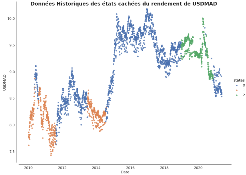
Chart 1: Hidden states of USDMAD pair returns

For the hidden states of the returns of the other 5 currency pairs, reference can be made to Chart 2 in the appendix.

The following comparison is made between the hidden states of the USDMAD pair: The zero state or “zero regime” with the highest average and the highest variance: it then represents our high volatility regime. Regime 1 is like our neutral volatility regime because its variance ranks second. And regime 2 is like our low volatility regime because its mean is ranked second and its variance is ranked last among the USDMAD hidden state variances. Thus, we can say that the GMM adapts better to non-stationarity on the USD/MAD pair. The GMM classifies returns into low, neutral and high volatility, giving for each group or regime its mean and its variance.

We can then generalize by saying that the GMM takes into account the non-stationarity of the 6 currency pairs.

4.2. Prediction of the evolution of yields

A return lying above the upper limit of the confidence interval of the Johnson Su distribution (1949) or the Gaussian distribution is called outlier too_high and will be called outlier too_low when it is below the lower limit the confidence interval of this distribution. A too_high outlier can be either negative or positive; A too_low outlier can also be either negative or positive. By exploiting the fact that the returns are generally close to zero, one can simply compare the sums in absolute value of the positive outliers and the negative outliers. If the ratio between the sum in absolute value of the positive outliers and the sum in absolute value of the negative outliers is greater than 1, this means that the returns are globally bullish, otherwise, they are globally bearish. The ratios in absolute value between the sum of the positive outliers and the sum of the negative outliers of the returns of the six currency pairs in the table above are greater than 1 and therefore show for this purpose that the returns of these currency pairs are in general bullish (see appendix, Table 2 for more details).

The calculation of the percentage of errors of the “correctly predicted” returns with the validation data can be paraphrased as follows: To evaluate our results globally, we have:

- Evaluate the forecast error of each currency pair for forecasts over 1 or 5 periods (days) ahead. In other words, we have evaluated the error of the forecasts of each currency pair at D+1 or D+5 in the future.

- Globally evaluate the forecast error of all the 6 currency pairs selected for the forecasts 1 or 5 periods ahead. In other words, we have globally evaluated the forecast error of all 6 currency pairs at Day+1 or Day+5 in the future.

Table 3: GMM with 4 factors or explanatory variables

	Model: GMM | Variable explained: exchange rate returns | Factors: TEDRATE, T10Y2Y, T10Y3M, T5YIFR | Data sources: Yahoo Finance and FRED | Number of components: 2 | Step: 1 or 5 | Lookback: 1 | Significance threshold: 1% | Cutoff: 2019 | start_date :01/01/2010 | end_date: 15/05/2021;
Currency pairs	USDZAR_lret	USDNGN_lret	USDEGP_lret	USDMAD_lret	USDMUR_lret	USDKES_lret
Degree of accuracy of the GMM	73,887%	66,766%	32,344%	61,721%	51,929%	51,632%
Sum of errors	88	112	228	129	162	163

Table 3 above presents the percentages of precision of the forecasts of the evolutions made on the six exchange rates studied in this article. These changes are explained on the one hand by past exchange rates (previous) and on the other hand by the following 4 explanatory variables: TEDRATE, T10Y2Y, T10Y3M, T5YIFR.

A sample of USDNGN currency pair returns from 01/01/2010 to 05/15/2021, shows that the GMM estimates USDNGN currency pair returns with an accuracy of 72.700% (To obtain this result, we used the 7 financial variables: DFEDTARU, DFEDTARL, EFFR, TEDRATE, T10Y2Y, T10Y3M, T5YIFR).

It can also be seen in Table 3 above that the GMM-HMM predicts the movement of the USDZAR pair with a high level of accuracy of 73.887%. This clearly shows that exchange rate returns are predictable and they do not follow a random walk.

We can then generalize by saying that returns on exchange rates do not follow a random walk (we also say that the Forex market is inefficient) if we predict them with models such as the GMM or GMM- HMM.

From the last paragraph of subsection 4.1 and from the paragraph above, we can state on the one hand that the assumptions made in subsection 2.1 (concerning GMM and yields) are validated and on the other hand, that we predict very well the future evolutions of exchange rate returns. And therefore, this explains the fact that our robot built from the GMM-HMM model generates overall positive daily profits.

See Chart 3 in the appendix for charts of return forecasts made on the other 5 currency pairs.

4.3 Measures of Investment Risk: Sharpe Ratio and Other Indicators

Table 4: Some Risk Measures on Currency Pair Prediction

Mesures	USDZAR_lret	USDNGN_lret	USDEGP_lret	USDMAD_lret	USDMUR_lret	USDKES_lret
Sharpe ratio	1.531	1.561	1.501	1.545	1.503	1.520
Market Beta	0.007	0.004	0.001	0.001	-0.002	0.014
Value at risk or VaR (0.05)	0.057	0.052	0.0502	0.054	0.051	0.044
Covariance VaR (0.05)	0.027	0.025	0.023	0.026	0.024	0.0213

Table 4 above shows that all the 6 currency pairs studied in this work have a Sharpe ratio greater than 1 and therefore their different expected returns would be greater than the risks incurred on these currency pairs for an investor. Although there is great volatility in these 6 currency pairs, this ratio shows us that the expected return on an investment in these pairs is positive. The market betas are very low and show that the returns on these currency pairs are weakly dependent on the Forex market (due to the correlation between the currency pairs or the multicollinearity between the currency pairs). This also means that the volatility on these currency pairs also depends on other variables such as macroeconomic indicators of monetary and fiscal policies.

The value at risk coefficients and the value at risk variance covariance matrix are very low (around 5%) and clearly show that the minimal risk that an investor is prepared to take when investing in these pairs currency is acceptable. (See appendix, Table 5 for other statistical risk measurement indicators).

Conclusion

This article was about building a Daytrading strategy by applying a Gaussian mixture model to the following six marginalized currency pairs: USDZAR, USDNGN, USDEGP, USDMAD, USDMUR and USDKES. After reviewing the financial literature, we believe that this is the first time in the financial literature that a robot built from the GMM-HMM and trading on African currency pairs (and running in real time 24/7 24 in the Forex market) was developed (coded) and published by researchers. The Gaussian Mixture Model (GMM) we use here is a Gaussian Hidden Variables Mixture Model (much like a model combining the Gaussian Mixture Model and the Hidden Markov Model or GMM-HMM) because we estimated the returns exchange rates assuming that these can be explained on the one hand by their past returns and on the other hand by macroeconomic variables. We found that the GMM-HMM estimates returns for the USDZAR currency pair with 73.887% accuracy and the USDNGN currency pair with 72.700% accuracy.

The generally positive performance of the trading algorithm (robot) that we developed during this article convinced us to open our trading robot to natural and legal persons.

Based on the results of our estimates and the validation of our assumptions by these results, we can confidently recommend the attraction of foreign capital by African states and the African private sector. For this, on the one hand, African states must supervise, facilitate and make more flexible the procedures for creating asset management and algorithmic trading companies, and, on the other hand, the African private sector must make the effort to trust these asset management (and algorithmic trading) companies to manage a part of their financial assets (even if it is only a very small fraction).

References

Adam Smith (1759); Theory of Moral Sentiments

Adam Smith (1776); Researches on the nature and causes of the wealth of nations

Akerlof, George A. “The Market for ‘Lemons’: Quality Uncertainty and the Market Mechanism.” The Quarterly Journal of Economics, vol. 84, no. 3, 1970, p. 488–500. JSTOR, https://doi.org/10.2307/1879431. In American slang, a lemon is a car that is found to be defective after it has been bought.

Ali El Attar. Robust estimation of mixing models on distributed data. Learning [cs.LG]. University of Nantes, 2012. French. <tel-00746118>

Arthur Charpentier: Time series forecasting models; UQAM, ACT6420, Winter 2011; May 15, 2012; charpentier.arthur@uqam.ca, url: http://freakonometrics.blog.free

Bank of International Settlement, (2004), BIS Quarterly Review – International banking and financial market developments.

Bank of International Settlement, (2019), Triennial Central Bank Survey-Foreign exchange and derivatives market activity in 2019.

Baum, L.E.; Petrie, T. (1966). "Statistical Inference for Probabilistic Functions of Finite State Markov Chains"

BIS Papers No 90; Foreign exchange liquidity in the Americas; https://www.bis.org/publ/bppdf/bispap90.pdf; March 2017

Carl Edward Rasmussen: The Infinite Gaussian Mixture Model; Department of Mathematical Modeling; Technical University of Denmark; Building 321, DK-2800 Kongens Lyngby, Denmark carl@imm.dtu.dk; MIT Press (2000); https://groups.seas.harvard.edu/courses/cs281/papers/rasmussen-1999a.pdf                

Chan Ernest and Belov Sergei and Ciobanu Radu, Conditional Parameter Optimization: Adapting a Strategy to Different Market Regimes (April 14, 2021). Available at SSRN: https://ssrn.com/abstract=3880643; https://papers.ssrn.com/sol3/papers.cfm?abstract_id=3880643; https://www.predictnow.ai/blog/conditional-parameter-optimization-adapting-parameters-to-changing-market-regimes/

David Guerreiro: FOREIGN EXCHANGE MARKET BASICS: Financial Techniques; Year 2015-2016 Paris 8 University; david.guerreiro@univ-paris8.fr

Davis, Mark, and Alison Etheridge. “Mathematics and Finance.” Louis Bachelier's Theory of Speculation: The Origins of Modern Finance, Princeton University Press, 2006, pp. 1–14. JSTOR, http://www.jstor.org/stable/j.ctt7scn4.5.

Demsetz, H. (1968). The costs of transacting. Quarterly Journal of Economics, Vol.82, 33-53.

Douglas A. Reynolds et al: Speaker Verification Using Adapted Gaussian Mixture Models; M.I.T. Lincoln Laboratory, 244 Wood St., Lexington, Mass. 02420; Digital Signal Processing 10, 19–41 (2000)

Eriksson, S. and Roding, C., (2007), Algorithmic Trading Uncovered - Impacts on an Electronic Exchange of Increasing Automation in Futures Trading, Royal Institute of Technology, Stockholm.

Eugène Fama: "Efficient Capital Market: a Review of Theorical and empirical Works", 1970

German, M.B. (1976). Market microstructure. Journal of Financial Economics, 3, pp 257-275

Hamilton, James D. “A New Approach to the Economic Analysis of Nonstationary Time Series and the Business Cycle.” Econometrica, vol. 57, no. 2, 1989, p. 357–84.

Hendershott, T., (2003), Electronic Trading in Financial Markets, IEEE Computer Science.

Jake Vanderplas: "Python Data Science Handbook "ESSENTIAL TOOLS FOR WORKING WITH DATA [2016]; [p. 476 to 488]

John B. Taylor (January 1999) “A Historical Analysis of Monetary Policy Rules”; p. 319 – 348; URL: https://www.nber.org/system/files/chapters/c7419/c7419.pdf

John B. Taylor, Discretion versus policy rules in practice (1993), Stanford University, y, Stanford, CA 94905

Johnson, N.L. (1949). "Bivariate Distributions Based on Simple Translation Systems".

Johnson, N.L. (1949). "Systems of Frequency Curves Generated by Methods of Translation"; https://www.jstor.org/stable/pdf/2332539.pdf

Jun Cai: A Markov Model of Switching-Regime ARCH; Journal of Business & Economic Statistics, Vol. 12, No. 3. (Jul., 1994), p. 309-316

Lars Peter Hansen: "Large sample properties of generalized method of moments estimators". Vol.50, No. 4 (July 1982) p. 1029-1054

Laurence Broze: Econometrics of finance and nonlinear time series; University of Lille 3; https://moodle.univ-lille3.fr/pluginfile.php/381970/mod_resource/content/1/Poly1_2016.pdf; 2016-2017

Laurence Broze: Scoring methods and risk management; University of Lille 3; https://moodle.univ-lille3.fr/pluginfile.php/392292/mod_resource/content/1/Credit2016.pdf; 2016-2017

Lexis Fauth: High Frequency Trading Modeling and Statistical Arbitrage; University of Lille I; Master 2 Mathematics and Finance Mathematics of Risk 2012/2013

Lofgren, Karl-Gustaf, et al. “Markets with Asymmetric Information: The Contributions of George Akerlof, Michael Spence and Joseph Stiglitz.” The Scandinavian Journal of Economics, vol. 104, no. 2, 2002, p. 195–211. JSTOR, http://www.jstor.org/stable/3441066.

Lovjit Thukral, Hélyette German et al: "A daily Trading strategy in the ETN space", summer 2013, journal of trading.

Markov, A. A. 1913. An example of statistical investigation of the text Eugene Onegin concerning the connection of samples in chains. (In Russian.) Bulletin of the Imperial Academy of Sciences of St. Petersburg 7(3):153–162. Unpublished English translation by Morris Halle, 1955. English translation by Alexander Y. Nitussov, Lioudmila Voropai, Gloria Custance and David Link, 2006. Science in Context 19(4):591–600.

Michael L. Halls Moore-"Advanced Algorithmic Trading" (2017); Professional Quant Trading Strategies With Advanced Statistical Techniques; Bayesian statistics, time series analysis and machine learning for profitable strategies.

Mundell, Robert A. (1963). "Capital mobility and stabilization policy under fixed and flexible exchange rates". Canadian Journal of Economics and Political Science.

Muth, John F. “Rational Expectations and the Theory of Price Movements.” Econometrica, vol. 29, no. 3, 1961, p. 315–35. JSTOR, https://doi.org/10.2307/1909635.

Patrik Idvall, Conny Jonsson; Algorithmic Trading: Hidden Markov Models on Foreign Exchange Data; LiTH - MAT - EX - - 08 / 01 - - SE

PREDICTION OF FINANCIAL TIME SERIES WITH HIDDEN MARKOV MODELS by Yingjian Zhang; B.Eng. Shandong University, China, 2001

Psychology of Great Traders, Thami Kabbaj (Author); Published in September 2011 Study (paperback)

R. Brealey, M. Myers et al: Principles of Financial Management; 8th edition; 2006

Robert Lucas, (1970), Capacity, overtime and empirical production functions, American Economic Review, 60, (2), 23-27

Rüdiger Dornbusch (1976). "Expectations and dynamics of the exchange rate". Journal of Political Economy. 84 (6): pp. 1161–1176.

Steve Renals and Peter Bell: "Hidden Markov models and Gaussian mixture models"; Automatic Speech Recognition— ASR Conferences 4&5 January 28/31, 2013;

Stiglitz, Joseph E. “Information and Economic Analysis: A Perspective”. The Economic Review, vol. 95, 1985, p. 21–41. JSTOR, https://doi.org/10.2307/2232867.

Taleb, Nassim Nicholas (2018). "Introduction". The skin in the game: hidden asymmetries in everyday life.

Thami Kabbaj: Psychology of Great Traders; Published in September 2011 Study (paperback)

The summation of random causes as a source of cyclical processes E. Slutzy 1927 Problems of economic conditions The Conjuncture Institute, Moscow vol 3 (1); published in English in Econometrica Vol. 5 (2) April 1937, p. 105-146

​​Tversky, A., & Kahneman, D. (1981). The framing of decisions and the psychology of choice. Science, 211, 453-458

Valérie Monbet - 2011: "Modelling time series", 2011. pp 30-39

Wald, A. and Wolfowitz, J. (1940), "On a test whether two samples are from the same population," Ann. Mathematical Statist. 11, 147-162.

Wang, Shixiong; Li, Chongshou; Lim, Andrew (2019-12-18). "Why ARIMA and SARIMA are not enough". https://arxiv.org/pdf/1904.07632.pdf

Noel, Udny. 1927. On a method of investigating periodicities in perturbed series with special reference to Wolfer sunspot numbers. Philosophical Transactions 226: 267-298.

Zeljko Ivezic, Andrew J. Connoly, Jacob T. Vanderplas, and Alexander Gray: "Statistics, Data Mining, and Machine Learning in Astronomy". A PRACTICAL PYTHON GUIDE TO SURVEY DATA ANALYSIS. Princeton University Press. [2014]. [p.134 to 139]

Zoran Zivkovic: Improved adaptive Gaussian mixture model for background subtraction; Intelligent and Autonomous Systems Group; University of Amsterdam, Netherlands; In Proc. ICRP, 2004

Annexes:

Figure 2: Hidden states of returns for other currency pairs

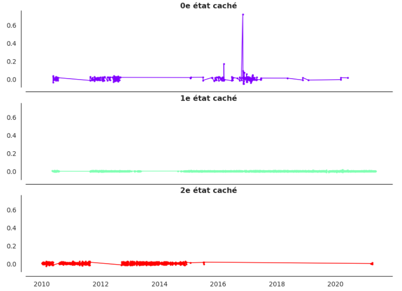
Case of USDZAR returns                                                                                          Case of USDNGN returns                                                                     Case of USDEGP returns                                                                                                         Case of USDMUR returns                                                                      Case of USDKES returns

Table 2: Some descriptive statistics of the outliers of the returns of the six currency pairs

	USDZAR_lret	USDNGN_lret	USDEGP_lret	USDMAD_lret	USDMUR_lret	USDKES_lret
Mean	0.0018	0.0048	0.0005	0.0003	0.0043	0.0031
Median	0.0027	0.0016	0.0003	-0.0008	0.0060	0.0040
Maximum	0.0213	0.0832	0.0133	0.0281	0.0306	0.0113
Minimum	-0.0228	-0.0142	-0.0087	-0.0096	-0.0137	-0.0145
Number of +	20	30	50	19	46	53
Number of -	10	4	38	25	19	16
Sum of +	0,1564	0,2261	0,0958	0.0922	0.3734	0.2860
Sum of -	-0,1015	-0,0235	-0,0482	-0.0796	-0.0926	-0.0684
Ratio of +/-	1,5399	9,6086	1,9849	1.1577	4.0335	4.1809
%+	0.6667	0.8824	0.5682	0.4318	0.7077	0.7681
%-	0.3333	0.1176	0.4318	0.5682	0.2923	0.2319

Number of +: number of positive outliers | Number of-: number of negative outliers | Sum of +: sum of positive outliers | Sum of-: sum of negative outliers | +/- ratio: ratio in absolute value between the sum of positive outliers and the sum of negative outliers | %+: percentage of positive outliers | %-: percentage of negative outliers | Parameters: a=0.2 and b=0.7 (obtained from finding Coarse parameters) | threshold=1% | Model: GMM | Explained variable: exchange rate returns | Factors or Explanatory Variables: DFEDTARU, DFEDTARL, EFFR, TEDRATE, T10Y2Y, T10Y3M, T5YIFR | Data sources: Yahoo Finance and FRED | Number of components: 2 | Step_fwd: 1 day | lookback: 1 year | Cutoff: 2019 | start_date:01/01/2010 | end_date: 05/15/2021;

Graph 3: Predictions of yields from validation data

Table 5: Some Measures of Risk on Currency Pairs

Measures	USDZAR_lret	USDNGN_lret	USDEGP_lret	USDMAD_lret	USDMUR_lret	USDKES_lret
Sharpe ratio	1.531	1.561	1.501	1.545	1.503	1.520
Market Beta	0.007	0.004	0.001	0.001	-0.002	0.014
The Treynor Ratio	124.254	-1973.573	-96.454	-100.605	72.307	56.637
The information ratio	-1.633	-1.384	-1.317	-1.922	-1.714	-1.722
Sortino ratio	1840.319	377.377	975.907	488.347	1037.127	166.322
The Omega Report	45689.408	14139.952	31179.686	7643.566	21025.002	8382.472
Kappa ratio 3	591.283	105.757	297.868	185.675	360.237	44.405
Value at risk or VaR (0.05)	0.057	0.052	0.0502	0.054	0.051	0.044
Covariance VaR (0.05)	0.027	0.025	0.023	0.026	0.024	0.0213

---